
The current Pleistocene Ice Age has heavily influenced the distribution of species. One could argue it still does – the Ice Age is not a thing of the past, we are now merely experiencing a relatively warm interval (called the Holocene). During an Ice Age, the climate cycles between long cold spells (glacial periods) and short warm spells (interglacials) and this temperature fluctuation is larger, further away from the equator. During the glacial periods many species had their ranges reduced in so-called glacial refugia, where conditions remained agreeable (whereas populations outside these areas went extinct). During interglacials they could expand their distributions again from these glacial refugia. This pattern of range reduction and expansion repeated itself with each climate cycle.

The three southern European peninsulas – Iberian, Italian and Balkan – played a major part as glacial refugia. Many temperate species in Europe had their current ranges reduced to one of these peninsulas during glacial periods and they colonized the rest of their current range from here as glacial conditions alleviated. The Carpathians are now increasingly being recognized as a relatively northern glacial refugium.
In stable populations in glacial refugia genetic diversity accumulates over time and, when they get isolated from one another, such populations diverge. On the other hand, postglacially established populations typically arise from a few founders that represent only a fraction of the total genetic variation present in a species. Hence, population stability and expansion leave different signatures in a species’ genes across its range. The late Godfrey Hewitt, thinking from a northern hemisphere perspective, dubbed this pattern “southern richness and northern purity”.

The genetic diversity for T. cristatus is high in the Carpathian region (two lower panels; mitochondrial DNA (left) and nuclear DNA show three main genetic groups, represented by different colors; populations in grey are genetically admixed with other crested newt species). However, genetic diversity is basically zero in the rest of its range (top panel; one genetic group only). In the lower panels the Carpathian mountain range is shaded grey.
As we strongly suspected that the crested newt Triturus cristatus provides a particularly extreme example of the “southern richness and northern purity” paradigm, we conducted a detailed screening of genetic diversity and investigated the distribution of suitable habitat at the height of the last glaciation. Several distinct genetic clusters occur in the Carpathians nowadays, whereas in the rest of its range T. cristatus shows extreme genetic depletion: newts from the UK and the Urals are indistinguishable based on the markers we studied! Most of the current range of T. cristatus was totally uninhabitable at the Last Glacial Maximum, but suitable area remained in the Carpathians. Our study, published in the Biological Journal of the Linnean Society, shows that most of the huge current range of T. cristatus was only colonized after the last glacial period ended, from a glacial refugium situated in the Carpathian region.

These ecological niche models show area predicted suitable for T. cristatus nowadays (top) and at the height of the last glacial period, the Last Glacial Maximum (c. 21,000 years ago).
Reference: Wielstra B, Babik W, Arntzen JW (2015). Postglacial recolonization of Europe by the crested newt Triturus cristatus from an extra-Mediterranean glacial refugium – the Carpathian region. Biological Journal of the Linnean Society 114(3): 574-587.
![]()
I conducted this work as a Newton International Fellow.
Note that the numbering of Fig. 2 in the original paper was off (thanks to Robert Kuipers for pointing this out). Here is a corrected version:
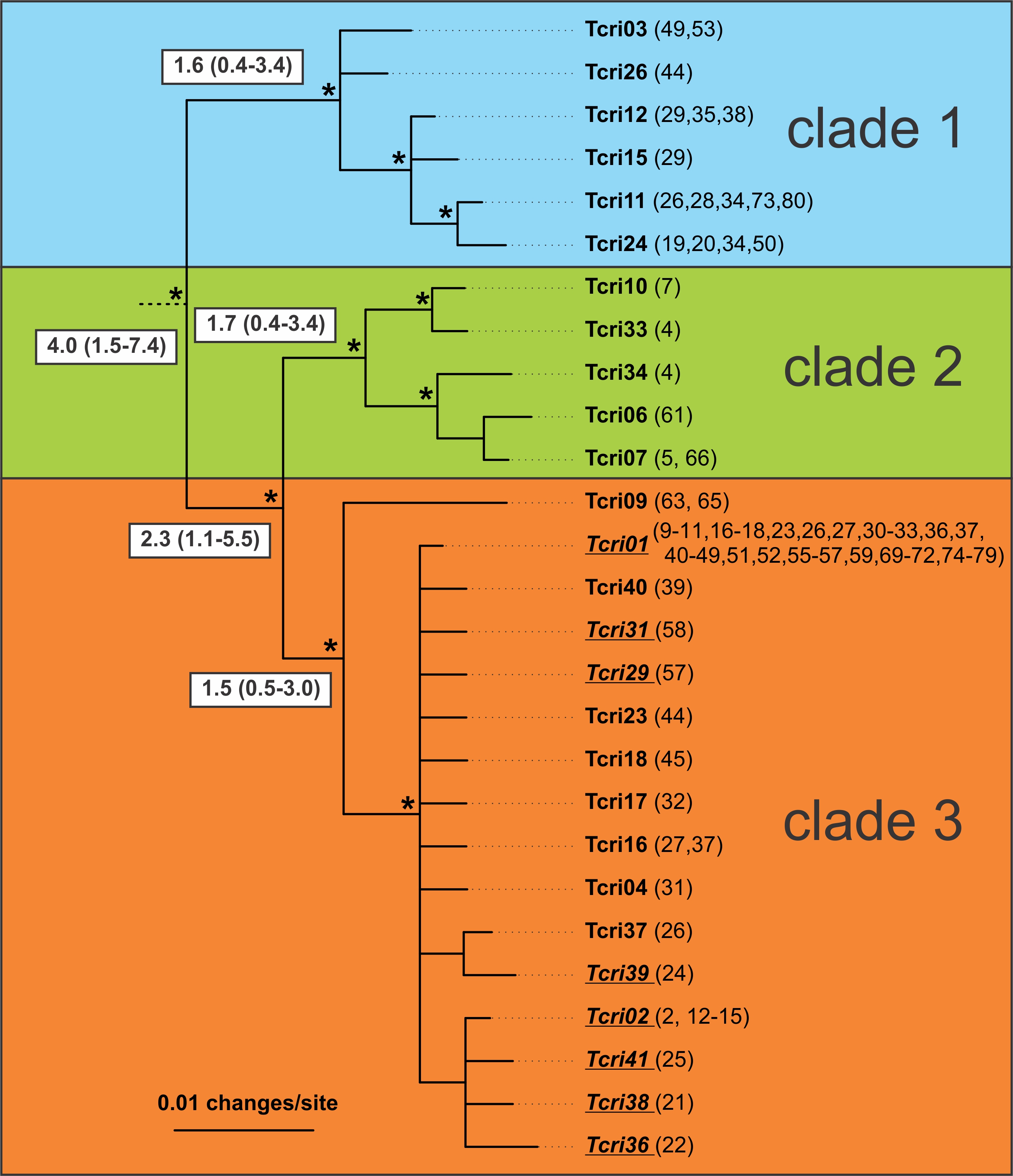
Another issue I noticed after publication is the placement of population 32. This should be more to the northwest and that makes much more sense actually. Here is the corrected figure:


I haven’t read the article, because it is paywalled, but I have some questions regarding this blog-piece:
Figure 2 in this text:
– Does every dot represent one or more salamanders?
– In the case of more salamanders: How many individuals does one dot stand for?
– In the case of one salamander: How are you going to explain the mtDNA figure down left where dots are half orange/blue, grey/green and orange/grey? That is impossible, because it immediately destroys MtDNA phylogenetic theory (Mutable at a constant rate)
– Do all orange dots stand for individuals that are genetically indistinguishable from each other in all three maps (figure 2)?
– “populations in grey are genetically admixed with other crested newt species” Can you explain which newt species please? I am also interested in the two grey dots seen in Austria: T. carnifex or T. dobrogicus perhaps?
– Did you also check the one mitochondrial protein-coding gene, three nuclear introns, and one major histocompatibility complex gene thoroughly in the populations of T. dobrogicus, T. macedonicus and T. ivanbureschi to rule out the possibility that these ‘foreign’ genes did ‘pollute’ T. cristatus populations in any way in the Carpathian region?
– How many specimens of these three populations did you check on these genes?
– For example you said that T. dobrogicus is both in MtDNA and nuclear DNA very diverse. Is there a clear difference between the eastern and western population of T. dobrogicus regarding the genes used for this research?
– Do we have a fairly solid picture of the genetic structure of T. dobrogicus?
– How can one know that T. dobrogicus has any pure species DNA left when it seems to hybridize with all the surrounding populations it comes in contact with? Same goes for T. cristatus in the Carpathian region.
– If so then where is the published research or does this article cover all of these problems?
– Could this ‘genetic richness’ in the Carpathian region be evidence that T. cristatus did indeed invade this very complex region after the Last Glacial Maximum (LGM) and interbred with the living and extinct ‘species’ of Triturus there and eventually displaced them leaving only traces of their DNA behind in its own DNA?
– Or that T. cristatus is a derivative of the genetically very diverse T. dobrogicus that evolved during the LGM or the LGM before that with the trait that this form is capable of rapidly dispersing across Europe unlike the other Triturus species?
That’s interesting, because it could easily explain why the T. dobrogicus distribution is split in two and it could also explain figure 3 in https://benwielstra.wordpress.com/2014/10/23/trying-to-crack-the-crested-newt-phylogeny-and-failing/ .
This last paragraph would also undermine the phylogenetic theory, because it implicates that genes are not mutable in time at a constant rate.
– Do you (as authors of the article) realize that you are just focussing on the LGM and that the Earth experienced some 15-20 glacial periods in the last 2.5 my with the last four glacials to be the coldest? That is a well established fact in paleoclimatology.


http://onlinelibrary.wiley.com/doi/10.1029/2004PA001071/pdf – figure 4
We don’t know how salamanders got through (evolutionary speaking) during these climatic roller-coaster rides. We do however know that birds and mammals radiated like crazy during these oscillations.
And we also do know that our understanding of glacial refugia is poor.
A quote from Hewitt 2000 (the source you referenced): “The present genetic structure of populations, species and communities has been mainly formed by Quaternary ice ages, and genetic, fossil and physical data combined can greatly help our understanding of how organisms were so affected.”
And Hewitt 2004 again: “Our poor understanding of refugial biodiversity would benefit from further combined fossil and genetic studies.”
The fossil record of salamanders (especially Triturus) is poor and to bet on genetics alone is not the way how science should advance. Hewitt at least recognizes that, but it seems that this blog and probably your article are hanging their hat on genetics only.
– If T. cristatus was present during the Pleistocene Era why did it not possess a refugium in France/Spain for example given the dispersing nature of the species during interglacials?
According figure 3 France/Spain are very good places for a glacial refugium.
– Perhaps more evidence that T. cristatus did indeed evolve during the LGM or that it completely merged with another species of Triturus living in France/Spain during the previous interglacial that has now become T. marmoratus? When one looks at the morphology (skin texture for example) of T. marmoratus there seem to be some features there of a cristatus like ancestor/combination.
– Do you in your article say specifically that MtDNA and nuclear DNA are behaving very differently when it admixes with DNA from other species?
A great example are wolves in Italy and the mixing with feral dogs. It seems that wolves can only breed and successfully raise their young in a certain period of the year. Unlike dogs estrus in female wolves only occurs in late winter. So in fact only male dogs will be able to mate with female wolves and successfully raise their offspring. (Wolves: Behavior, Ecology, and Conservation by Mech & Boitani 2003)
– Will MtDNA from the offspring in such a population of wolves reveal mixing with feral dogs? (no need to answer – rhetorical question)
One last remark.
Your quote: “In stable populations in glacial refugia genetic diversity accumulates over time and, when they get isolated from one another, such populations diverge.”
There is a beautiful isolated species living in Europe for quite some time (so it seems) with a fairly large distribution according the literature in a mountainous area. It should resemble somewhat of a refugium at the time of a LGM.
– 5 my according Steinfartz et al (2000)
– 3.5 my according Vences et al (2014)
I am talking about Salamandra corsica here.
If the hypothesis of the late Godfrey Hewitt and your quote are right we should see a large genetic variation in this species. My suggestion would be to do a comparative research on this species using the one mitochondrial protein-coding gene, three nuclear introns, and one major histocompatibility complex gene combined with a morphological study to establish if you and Hewitt are right after all.
Greetings,
Robert
Dear Robert,
I have sent you the paper as this will clarify at least most of your questions. Please post remaining questions if any here in a concise manner and I will see if I can answer them.
Cheers,
Ben
– Why is Tcri01 (orange clade) designated as a blue clade in the map figure 1B? Numbers 19 – 28 – 34 – 50 – 53 – 73 – 80 are all blue when they should have been orange to my opinion.
– Where are numbers 81 and 82 on the map? (Figure 2 Tcri01 (77-82))
– How is it possible that Figure 1 B Clade 2 has so many introgressed MtDNA genes while we see very few hybrids in figure 1 C?
– And which nuclear genes (βfibint7, CalintC or Pdgfrα) are the ‘foreign’ ones in these specimens? Numbers 5 and 61.
– Why did you not exclude the hybrids or introgressed specimens in the entire research? It gives a confusing picture.
“A fossil dated at 24 Mya was interpreted
as a minimum estimate for the most recent common
ancestor of the genus Triturus and was appointed a
lognormally distributed prior with a mean of 24,…”
You or your colleague used this fossil earlier in other research.
– Can you give more specifics about this fossil please? Where can I find it? What fragments?
I have more questions and will be back later.
– Fig. 1A is colour coded according to mtDNA, Fig. 1B according to nuDNA. nuDNA and mtDNA show slightly different distribution.
– You have pointed out an unfortunate error in numbering in Fig. 2 that I missed. Well spotted. It caused a mismatch in numbering. Raw data is in appendix 1, please refer to that for mtDNA distribution. Fig. 1 is correct.
– An initial hybridization with repeated backcrossing will dilute out nuDNA over the generations. Another way of stating this is that the species with which backcrossing occurs is reconstructed. The less markers you study the lower the chance you will pick up remnants of past hybridization. As we only study three markers and backcrossing has been possible for many, many generations we do not pick up traces of ‘foreign’ nuDNA. mtDNA does not recombine as does nuDNA, instead it is transmitted clonally. Furthermore, due to less intraspecific gene flow it is less susceptible to genetic swamping. As a consequence, mtDNA is relatively susceptible to introgress. For more information see Petit, R.J., Excoffier, L. (2009): Gene flow and species delimitation. Trends Ecol. Evol. 24: 386-393.
– You can compare appendix 1a and 1c to determine introgressed alleles. E.g. for the individual from population 5 allele PDG38 is not found in other T. cristatus but widely distributed in T. dobrogicus
– Hybrids were excluded because they do not represent the (entire) evolutionary history of T. cristatus. Hybrids would have inflated genetic diversity and provide a misleading picture on the evolution of intraspecific genetic diversity.
– For the calibration point see: Steinfartz, S., Vicario, S., Arntzen, J.W., Caccone, A. (2007): A Bayesian approach on molecules and behavior: reconsidering phylogenetic and evolutionary patterns of the Salamandridae with emphasis on Triturus newts. Journal of Experimental Zoology Part B: Molecular and Developmental Evolution 308B: 139-162.
“- You have pointed out an unfortunate error in numbering in Fig. 2 that I missed.”
I am not only speaking of the numbers 81 and 82.
I checked with Appendix S1 and see results below:
Pond nr. Tcri number(s)
19 24
28 11
34 11, 24
50 24
53 03
73 11
80 11
Figure 1 is correct, but figure 2 is incorrect (Tcri01). Pond numbers belong to blue clade.
– “An initial hybridization with repeated backcrossing will dilute out nuDNA over the generations.”
I agree with this, but it should also dilute out MtDNA over the generations because of high mortality and lower fitness of the hybrids. The abundant observation of admixed MtDNA of T. ivanbureschi therefore is way too high.
Your argument/reasoning can only work when the hybrids (only the females) are very fit to reproduce. Do you have evidence for that, because most literature claims otherwise?
If you are right it would mean that the fitness of the F1/F2 etc females is very high.
For two species that split up 10-11 Mya in the case of T. cristatus and T. ivanbureschi it is very peculiar to produce such fit offspring.
I can’t get a full copy of Petit et al 2009: Gene flow and species delimitation. Will you be able to send me a copy perhaps?
– “allele PDG38 is not found in other T. cristatus but widely distributed in T. dobrogicus”
Sorry that is something I cannot determine with the info (Appendix S1 and S2) that you sent me.
What research does reveal that PDG38 is widely distributed in T. dobrogicus or nuclear alleles from other Triturus species? This article and Appendices do not.
– Exclusion of hybrids: I have read the same response in your article. You did not understand the question so let me rephrase it:
Why do I still find PDG38 for example in the Phylogenetic tree of Appendix S2?
Why do I still see a lot of grey dots in Figure 1B for example?
That I find very confusing.
– Calibration point: Steinfartz et al 2007 uses Estes 1981 as a source:
“C4 corresponds to the crown of the
large-bodied Triturus (LBT) (crested and marbled
newts), which should be older than the Lower
Miocene fossils of Triturus, cf. T. marmoratus
(Estes, ’81), dated to 24.2–23.8 mya (Bohme,
2003).”
It looks like there is no actual fossil dated at 24 mya. There is only a T. marmoratus fossil from the lower Miocene. The date (24 mya) looks to be an estimate.
Ectothermic vertebrates (Actinopterygii, Allocaudata, Urodela, Anura, Crocodylia, Squamata) from the Miocene of Sandelzhausen (Germany, Bavaria) and their implications for environment reconstruction and palaeoclimate – Bohme 2010
“Material examined: 15 atlas (16307), 183 trunk vertebrae
(6512, 6519, 6520, 16308, 16309), 3 occipital bones
(16310–16312), several cranial and postcranial remains
(16313).” from three different findings – all T. marmoratus fragments.
– Yes, the numbering of Fig. 2 is completely messed up, I am embarrassed I did not detect this before, I will post a corrected version here.
– mtDNA does not dilute, the mtDNA type present in the mother (and not the father) is transmitted to her offspring. It makes no sense to say the observed occurrence is too high, this is just how it is and what needs to be explained. Note that mtDNA introgression is regularly observed in crested newts, introgression of T. ivanbureschi mtDNA in T. macedonicus is much more extreme still! Indeed the fitness of hybrids cannot be zero, but because the transition between the species based on nuDNA is still pretty sharp (see the 2014 BJLS paper with Pim as first author) it appears fitness is lower than ‘purebreed’ newts. I think demography plays an important role. During initial colonization of ‘empty’ areas species obtain secondary contact and have little option in terms of mating. mtDNA introgression can occur at low initial frequency but because of allele surfing can end up covering a large area (see also Currat et al 2008 Evolution). Please note that one of the main reasons we study Triturus is because they are at this interesting stage in the speciation process where they still hybridize. I don’t think the timeframe is weird for amphibians. I have not conducted breeding experiments but some stuff has been done in the 1950s. It would be great if somebody could do such experiments in more detail.
– The appendix shows the genotypic data for the other crested newt species used to determine genetically admixed individuals. Hence, by comparing genotypes of admixed newts to both cristatus and the species with which admixture is observed you can deduce which alleles are typical of cristatus or the other species.
– Fig. 1B simply shows where admixture is observed. The phylogenetic trees show all alleles. These trees are presented for completeness sake. We argue that they are not an informative way to determine the evolutionary history. The main cluster based analysis excludes admixed newts. The results of this analysis are shown on Fig 1 in colours. So grey represents admixed newts not included in any of the coloured groups because they were excluded from the analysis.
– The fossil was used here to set the date of the crown of Triturus to 24Mya or older (interpreted as minimum age etc., the crown must be older than the T. marmoratus lineage). Note that Steinfartz used multiple independent calibration points and showed that the dating appears to be a good estimate.
(corrected Fig. 2 now posted above)
– “mtDNA does not dilute, the mtDNA type present in the mother (and not the father) is transmitted to her offspring.”
That’s true and that was not what I meant. On the individual level it cannot dilute out like nuDNA does, but on a population level it could if more and more genuine females of the invading species also take part of the hybridization process.
But that is not what seems to be the case with T. cristatus and T. ivanbureschi as far as I can read. Asymmetric breeding seems to be a factor.
– Now here is a problem with clade 2.
In samples from pond 4-8 there are three TkarC haplotypes (sample ID 4755, 4733 and 2612) with nuclear BF01 and also three Tcri haplotypes (sample ID 4754, 4756 and 4784) with BF01.
BF01 is not present in any more samples from the raw data.
Now how can you determine if these BF01 haplotypes belong to either TkarC or Tcri judging from the raw data only? You obviously assign BF01 to Tcri.
BF01 could be a foreign gene as well and not belong to Tcri at all. So therefore the sample IDs 4754, 4756 and 4784 could be admixed specimens as well and therefore should all be grey instead. Just like sample ID 4785 which is considered to be admixed.
Here is another interesting article: Polar and brown bear genomes reveal ancient admixture and demographic footprints of past climate change by Miller et al 2012.
From the site of Jerry Coyne: https://whyevolutionistrue.wordpress.com/2012/07/24/a-new-study-of-polar-bears-underlines-the-dangers-of-reconstructing-evolution-from-mitochondrial-dna/
mtDNA of one type can only ‘dilute out’ if mtDNA of another type comes in. However, once mtDNA has introgressed at the frontier of a colonizing species, that species will spread the introgressed mtDNA when it further expands (the introgressed mtDNA surfs the expansion wave).
Identification of admixture is based on analysis of the three nuclear markers together. Some alleles might not be informative here. Arguably three markers is a low number, particular if variation within these markers is high so ancestry determination is hampered as in the example you mention. Yet the data still appears to be quite powerful and I have found no obvious contradictions when analysing a much larger number of less variable markers (preliminary analyses of unpublished data).
Although I am a loyal reader of Jerry Coyne’s website I somehow missed the bear post so thanks for highlighting it. You can see mtDNA introgression as a disadvantage, but as I have argued before you can use it to your advantage as it provides insight into e.g. historical biogeography: http://www.biomedcentral.com/1471-2148/12/161 By the way, more bear gene flow recently published: http://www.molecularecologist.com/2015/02/threat-down-gene-flow-from-polar-bears-into-brown-bears/
Thanks for the two polar bear articles by Cahill et al. Always welcome in my library. By Cahill et al 2015:
“Two studies, Miller et al. 2012 and Liu et al. 2014; have also attempted to estimate the time of population divergence from whole genome data using populationmodelling frameworks. Liu et al. estimated population divergence to have occurred 343–479 thousand years ago with postdivergence gene flow from polar bears to brown bears (Liu et al. 2014). Miller et al. estimated a much earlier 4–5 million years ago divergence followed by bidirectional postdivergence gene flow (Miller et al. 2012). Given the greater concordance of the 343–479 thousand years ago population divergence with other genetic divergence estimates it appears to be a better supported.”
That’s a whopping 3.7-4.7 million years difference of estimated population divergence between both studies.
You said earlier in this discussion:
“You can compare appendix 1a and 1c to determine introgressed alleles. E.g. for the individual from population 5 allele PDG38 is not found in other T. cristatus but widely distributed in T. dobrogicus”
I have been searching in your publication list to find out if that was correct and I found the article http://www.sciencedirect.com/science/article/pii/S1055790313000286#fx1 As far as I know the only article in your list that deals with the PDG38 marker or I must have overlooked another one.
6 specimens (out of 50 samples or so) of T. dobrogicus had the PDG38 marker in its distribution range. And yes you are fairly correct with your statement that it is ‘widely’ found in T. dobrogicus. Case closed one might think.
Now I noticed something very peculiar in figure 3 (Pdgfra) of that multimarker article (Multimarker) when I compare it with figure 4 (Pdgfra) of the article discussed in this blog (Refugia).
PDG23
In figure 4 (Refugia) PDG23 is 7 bars away from PDG38 –
In figure 3 (Multimarker) PDG23 is 15 bars away from PDG38.
PDG25
In figure 4 (Refugia) PDG25 is 8 bars away from PDG38 –
In figure 3 (Multimarker) PDG25 is 18 bars away from PDG38.
PDG21
In figure 4 (Refugia) PDG21 is 7 bars away from PDG38 –
In figure 3 (Multimarker) PDG21 is 15 bars away from PDG38.
PDG24
In figure 4 (Refugia) PDG24 is 7 bars away from PDG38 –
In figure 3 (Multimarker) PDG24 is 15 bars away from PDG38.
PDG46
In figure 4 (Refugia) PDG46 is 9 bars away from PDG38 –
In figure 3 (Multimarker) PDG46 is 13 bars away from PDG38.
PDG30
In figure 4 (Refugia) PDG30 is 7 bars away from PDG38 –
In figure 3 (Multimarker) PDG30 is 11 bars away from PDG38.
I just counted the substitution bars that were notably seen in both figures and took the shortest route to PDG38. If we are actually dealing with markers (empirical and testable data) here the difference can’t be so big between the various markers when compared with PDG38. The result in constructing a network diagram should be exactly the same in both cases. Can you explain why there is so much difference in substitution bars between the two figures? And why is PDG38 in figure 3 (Multimarker) situated outside of the T. cristatus markers while in figure 4 (Refugia) it is literally inside the T. cristatus diagram?
Even though of course the distance between the haplotype pairs is identical, it is not so that the network analyses should show the same number of steps between them. The Refugia network only shows haplotypes sampled in T. cristatus. The Multimarker network on the other hand shows haplotypes sampled in all crested newt species.
Pingback: Carpathian ‘refugia-within-refugia’: evidence from two newts | Ben Wielstra